
Dynamical Modelling with Neural Differential Equations
Meeting Halfway: Between Dynamical Modelling and Data Science
There are two fundamental ways how we can try to understand dynamical phenomena in Nature. The traditional one is based on mathematical modelling. We look at the system of interest, strip away “all unnecessary features” whose contributions to the dynamics are “of lower orders” and build a mechanistic model under these simplifying conditions. Such models can be very powerful for qualitative understanding of mutual interactions between the actors in the system, but due to the simplifications, quantitative predictions might deviate from reality. An example from physics could be the Ising model of magnetization. In its simplest 2D form, the microscopic magnetic moments (spins) are placed on a two-dimensional lattice and only short-range (nearest-neighbor) interactions are considered. Thus, the minimal-energy state is associated with all spins aligned, i.e., a ferromagnetic state. By introducing temperature \(T\) , the system starts to be exposed to thermal fluctuations which increase with \(T\), and at some point they might completely break the ferromagnetic order. If one follows the mean magnetization over the ensemble of individual spins with Boltzmann distribution, one finds that there is a second-order phase transition at certain critical (Curie) temperature \(T_c\) where magnetization completely disappears. This phenomenon is indeed observed in natural ferromagnets and the Ising model gives a good understanding of the competition between the spin-spin interaction enforcing magnetic order and the thermal noise acting against it. From the model, one can also deduce the critical temperature \(T_c\). Its value, however, is difficult to link directly to real materials since too many simplifications were used.
Systems biology represents a similar mechanistic approach. The regulation of a target gene \(Y\) via a transcription factor \(X\) is often linked through the Hill function. This relation is derived from mass action kinetics and does not take into account any detailed biophysical features of the DNA binding. As a result, there is a simple relation from \(X \to Y\) with only a few parameters (concentration of \(X\), promoter strength and degree of cooperativity). With this obviously simplified approach one can already build principles of gene regulatory networks and understand the designs of network motifs and their function. On the other hand, direct quantitative predictions for complex biological systems are still limited.
A different way is to learn our insights purely from statistical analysis of the data that we collect from the system. Over the past two decades, this approach has become increasingly important across many research fields, thanks to major improvements in how we collect large data sets. In molecular biology, this has been represented, for example, by the development of sequencing technologies that generate genome-wide data, now also with single-cell or spatial resolutions. A lot of development has beed done on optimisation of statistical methods and tools for analysis of such data. The growing demand for more quantitatively trained researchers has drawn many of us—from traditional systems biology, computer science, or physics—into the fields of bioinformatics and computational biology (myself included). Statistical inference can answer important questions like “which genes are differentially expressed upon treatment”, or “what are the putative ligand-receptor interactions that drive the observed transcriptional changes”, but it does not provide direct mechanistic understanding.
There can, however, be a third way trying to meet half-way between the world of mathematical modelling and data science. The idea is to use the existing models that contain already lots of knowledge about the system, and use data to either improve the model’s predictive capacity or to adapt it for a certain task (e.g., control problems). This approach is known as Scientific Machine Learning (SciML) and a path to it was paved mainly by this paper introducing Neural Ordinary Differential Equations (neural ODEs). The core observation in the paper was that so-called residual networks (ResNets), which were originally introduced to deal with vanishing gradient problems during training, actually have the same structure as the Newton’s method of a numerical solution of an ODE. Thus, if one stacks “infinite” number of these layers in the network architecture, all these layers can be replaced by the ODE itself. This step brought dynamical modelling and machine learning onto a same platform, making it possible to combine differential equations with neural networks seamlessly.
Here, I will introduce two projects that use SciML for optimal control and model discovery.
Optimal Control Problems
Optimal control problems aim to map states of the system to the most optimal sequence of “pulses” (or other controllable interactions with the system) to fulfil certain pre-defined task. One example is reinforcement learning, where the interaction between an agent and its environment is modelled as a Markov decision process, and the optimal policy is found by maximizing the expected reward. In the formulation of the problem, there is no explicit model of the environments, so the agent must “learn the rules” purely in a data-driven way from its interactions with it. This makes the approach on one hand very general (no need to know anything about the system), but also very difficult to train – it’s very resource hungry-.
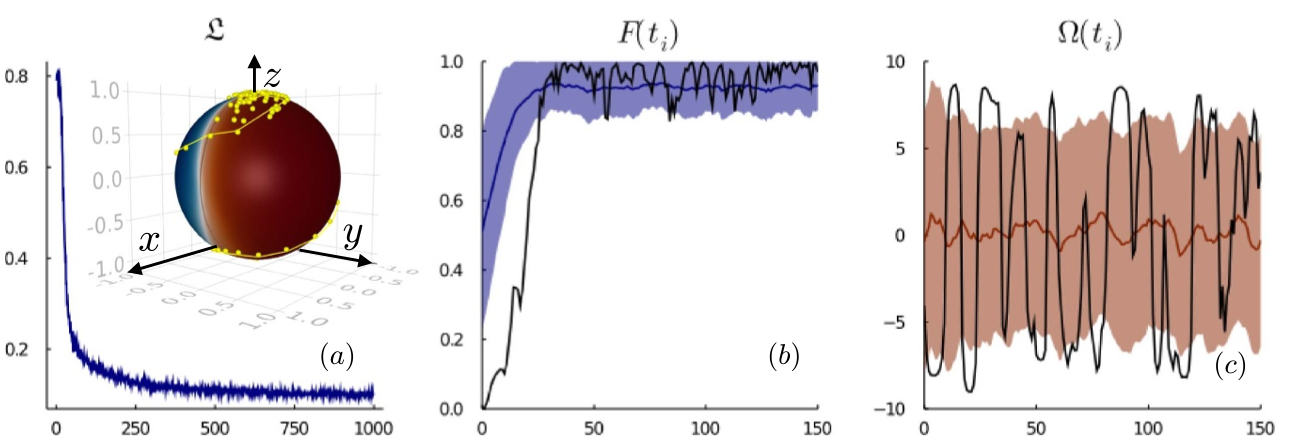
But in many cases there is a model that “reasonably well” reflects the dynamics of the problem. Thus, we use it and train the controller within the restrictions of the model. That is what we did when we thought of ways how to automatize state preparation for quantum computations. We investigated the problem in two control tasks: single qubit initiation (see Figure 1) and so-called cat-state preparation. First, we considered only deterministic dynamics (ODEs), later we also added effects of noisy measurements and learnt how to control stochastic dynamics as well.
See the original publications:
If you want to learn more about quantum computation, perhaps check my lectures.
Decoding ER\(\alpha\)-GATA3 Regulation in ER-positive Breast Cancer
Breast cancer (BC) is the most frequent cancer among women. One in eight women will develop the disease in their lifetime. Fortunately, up to 80\% of the cases are so-called ER-positive where cancer proliferation is dependent on signalling via estrogen receptor (ER) making is a suitable target for therapies. Clinically successful therapies contain selective estrogen receptor modulators (SERMs), degraders (SERDs), and aromatase inhibitors. Their use depends on patient’s clinical status. However, resistance can develop during treatment. Thus, understanding the details of ER signalling remains important to identify further therapeutic vulnerabilities.
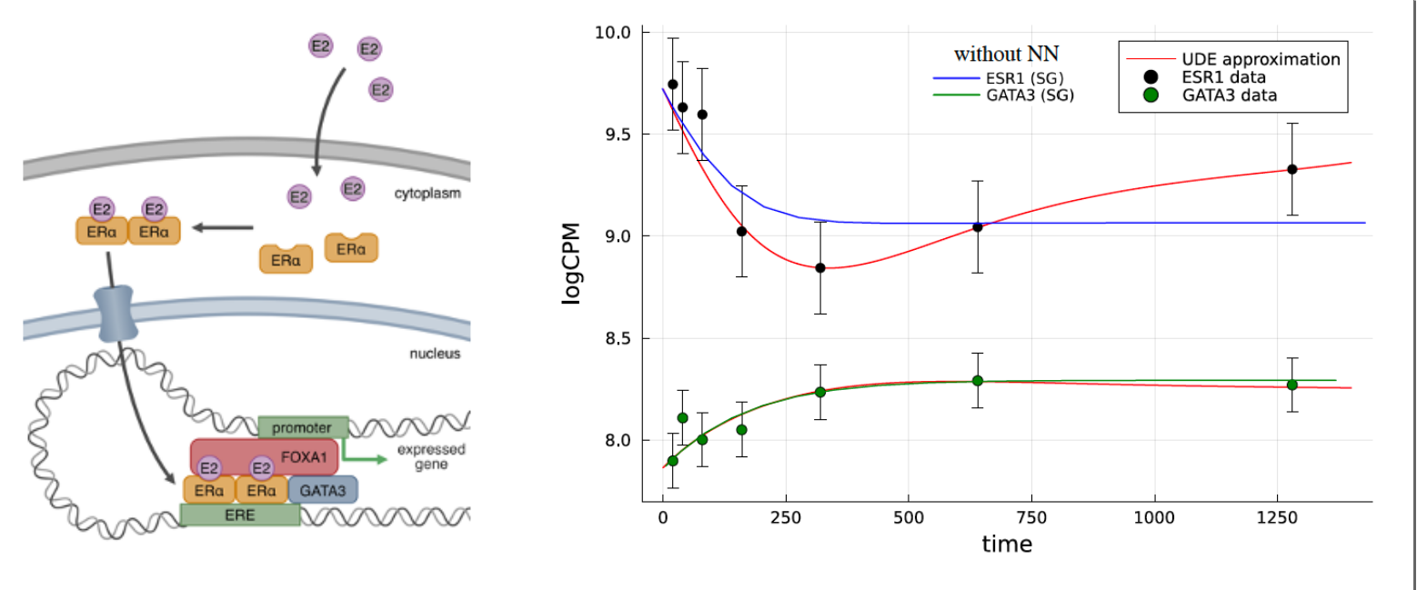
ER is a nuclear receptor (see Figure 2) which upon ligation by estradiol (E2) dimerizes and relocates to nucleus where it starts its transriptional program. Multiple co-factors are needed for the signalling. The most important ones are FOXA1 and GATA3. It has been reported that GATA3 co-regulates expression of ER in a form of a negative feedback loop. There were also attempts to quantitatively model this relation using multiplicatively-coupled feedback loops. However, the fitted parameters often lacked plausible biological meaning. As an example, in the above mentioned Hill functions, the cooperativity parameter \(n\) can be directly linked to the structures of the transcription factors; since ER forms dimers \(n = 2\), while GATA3 is a monomer \(n = 1\). When these parameters are fixed (and some others as well), a simple ODE-based model with multiplicatively-coupled feedback loops cannot fully reflect the dynamics. So the model perhaps misses some piece of the dynamics. The idea is to try to learn this missing piece from the data with an approach that is sometimes called Universal Differential Equations (UDEs) but basically it’s a synonym for neural ODEs for this specific application. In the first step the “traditional” mechanistic model is fitted to the data. In the next step a small neural network (NN) is added to the ODE model according to an educated guess. In other words, one examines the equations to identify where important dynamics may be missing. Then, the NN is initiated with small weights (we are learning possibly small corrections) and the system is retrained with the parameters from the original ODE already fixed. The result is shown in Figure 2 as well.
The procedure normally does not end here, since one might not be so impressed in the end that a highly parametrized NN that we added to the ODE can approximate “nearly any dynamics”. The final goal is to find an algebraic representation of the NN and thus to learn a mechanistic model of the dynamics that can, indeed, be written as a standard ODE, solved, and tested on parameter perturbations (for instance). To that end, one usually implements sparse regression algorithms like SINDy. In biological systems things are a little more complicated, so one needs to use the implicit version of this algorithm.
I have presented some preliminary results on recent conferences, the slides can be found here
A perfect reading on this topic is PhD thesis of Patrick Kidger.
I hope more updates will come in the near future!